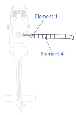
Helicopter modeling and simulation

Software is used to model and simulate helicopter behavior for several reasons. Computationally intensive CFD models may be used to study and improve airfoil shapes. Such models may even be coupled with acoustic software to predict rotor noise. Other, less computationally intensive models may be used to estimate high-level performance values like range and hover ceiling. Some models can be used to develop control laws and be incorporated in real-time simulators to train pilots.

In this article we’ll discuss what’s called comprehensive flight dynamics models. Such models incorporate enough aerodynamics and dynamics to provide useful predictions of rotor response, performance and handling qualities. They are sometimes used to test control laws in early stages of helicopter design. They incorporate sub models of dynamics and aerodynamics of the rotors, fuselage, landing gear and stabilizing surfaces. These subsystems are analyzed to varying degrees of fidelity. These models may be used in real-time flight simulators.

We’ll start with descriptions of the subsystem models: the fuselage, stabilizers, landing gear and rotors. After that, we’ll discuss how the outputs from these subsystems are put together in the overall model. We will then cover some useful processes normally included in a comprehensive model. Finally, we’ll cover the software engineering behind such models.

Subsystems

In this section, we’ll discuss models for each of the subsystems. Each model outputs at least six values: 3 forces and 3 moments at/about a stationline, buttline and waterline associated with the component. Internally, these models typically use one or more subsystem-specific reference frames. However, the output should be in high-level body attached frame.

You’ll notice a disparity in the complexity of these subsystem models. Rotor models are much more complex than others.

Fuselage Modeling

The structural deformations of a helicopter fuselage are rarely included in these models. Good approximations can be obtained without such details. Fuselage aerodynamics, however, must be included for useful simulations. A simple table lookup method is sufficient and often used to calculate these aerodynamics and will be described here. Other models use equations based on size and other geometry parameters. Rarely, the Navier-Stokes equations may be solved using a detailed specification of the fuselage geometry. The latter is very computationally intensive and avoided in most cases.

A table lookup model requires six input tables: three for forces and three for the moments. A reference point (stationline, buttline and waterline) where these forces and moments are applied is also input. Other inputs may be provided to govern rotor interference effects (e.g. in hover main rotor downwash on the fuselage can increase power required by 3%). The outputs are three forces and three moments in some body-attached frame, at/about the input reference point.

The input tables are two-dimensional, parameterized by fuselage angle of attack \(\alpha\) and sideslip \(\beta\). Mach number is typically unnecessary. Interpolation methods are used to determine aerodynamic coefficients \(c_i(\alpha ,\beta )\) from the table values. The coefficients - the table values - are typically normalized by dynamic pressure \(\rho v^2/2\), but not by size (unlike airfoil tables). Hence the \(i\)th force or moment \(F_i\) is simply computed as $$\begin{equation} F_i = \rho v^2 c_i(\alpha ,\beta )/2. \end{equation}$$

Stabilizer / Fin Aerodynamic Modeling

The same source code is typically used to model a horizontal stabilizer and vertical fin. Dynamic inputs include the free stream velocity at one or more points on the surface, atmospheric properties and optionally information about the rotor(s) and/or fuselage. The latter inputs may be used to model interference effects, i.e. changes in the airflow due to the rotor / fuselage. One or more velocity vectors are computed in a frame local to the surface. As with the fuselage, tables of lift, drag and pitch moment coefficients are typically used. An angle of attack is computed from the local velocity vector and coefficients are interpolated from these tables. Finally, the coefficients are scaled to forces and moments, which are eventually translated to an aircraft body reference frame.

Fuselage and rotor interference models may be based on a handful of empirically-derived equations or computed using e.g. free or prescribed wakes. Empirical parameters are based on the geometry of the specific aircraft. These interference effects should not be overlooked. For example, main rotor downwash on a horizontal stabilizer can substantially affect pitch behavior both statically and dynamically.

Modeling Controls

Control models output the feathering angle at the root of each blade. They also need to output the horizontal stabilizer angle for helicopters that have active stabilizers. Depending on the helicopter, these may be a simple function of the control stick position only (so-called direct control), or they may be a complex function of the control positions, flapping, flight dynamics and other things.

The simplest rotor control model is a linear, uncoupled direct control. In this model, the collective stick controls only the main rotor collective pitch, the F/A cyclic stick only 1/rev sin pitch variation, the lateral cyclic stick only the 1/rev cos pitch variation, and the pedals only the tail rotor collective pitch. The feathering angles are a linear function of the stick position.

Larger helicopters may include mixers and stability augmentation systems that complicate rotor controls. Control mixing may be implemented in a straightforward way, but SAS, SCAS and general AFCS behavior can be quite complex. Such complicated behavior is typically modeled in a separate subsystem which may be autogenerated by Simulink.

Passive control inputs like pitch-flap coupling are normally implemented in the rotor model. The rotor model may also include pitch change along the length of a blade due to flexing under loads, sometimes called elastic twist.

Unintentional feathering changes due to flexibility in the airframe and mast are typically neglected.

Practical swashplate systems have inherent nonlinearities. These result primarily from the motion of the pivot points or attach points used to convert linear motion to angular motion or vice versa. These effects are typically neglected as well.

Rotor Models

A sophisticated model is required to usefully simulate the main rotor for handling qualities and performance. Aspects of how blades flap and flex must be captured along with the impact on aerodynamics. The high frequency oscillatory aerodynamics of a blade in forward flight necessitates some level of unsteady aerodynamics. Reasonable performance predictions require a sophisticated wake model coupled in this analysis. A handful of methods may be used to perform this aerodynamic and structural dynamic analysis. Herein, we’ll discuss methods that yield useful predictions, yet can run in real-time on a workstation.

The model we discuss here is a blade element model, which treats elements of the blade (mostly) independently. A blade is typically subdivided span-wise into 5-20 elements as shown in the diagram below. The structural dynamics model will estimate the deflection and velocity of each blade element, including blade flexibility. The aerodynamics model will compute the airloads on each blade element, typically just lift, drag and pitching moment. The submodules will be further described below.

Structural Dynamics

A modal technique may be used to estimate blade dynamics. In this approach, 2 - 20 modes are input for a rotor. Each mode \(m_i\) includes flap-wise, chord-wise and twist displacement of all blade elements on the rotor, i.e. 3 DOF blade segments. The net displacement of all blade elements is a linear combination of these mode shapes \(\Sigma_i p_i m_i\). The coefficients \(p_i\) of this linear combination are called mode participation factors. They are time-varying values, computed in the model as a function of the loads on all blade elements.

The frequency \(f_i\) and inertia \(I_i\) of each mode shape are also provided as input. Since these values and the mode shapes depend only on the rotor design and rotor speed (not on the flight condition) they are typically computed by other software. The comprehensive flight dynamics software reads in these values from the output of the other software. If the comprehensive model needs to simulate a wide range of rotor speeds (rare), then it may need to read additional modes and include some method of interpolating all the mode information as a function of rotor speed. This may be required to simulate autorotations.

A reference for the differential equations of motion of a helicopter rotor blade is NACA Report 1346 by Houbolt and Brooks. We also provide a higher level introduction to rotor modes here. The comprehensive model computes the second time derivative of the mode participation factors \(p_i\) as \(\ddot{p_i} = W_i/I_i -2f_i d_i\dot{p_i} -f_i^2p_i\) and numerically integrates those to get elastic velocities and displacements of the blade elements. \(W_i\) denotes the virtual work on the \(i\)th mode and \(d_i\) is a sometimes useful modal damping value.

In addition to the aerodynamic loads, there are inertial loads acting on the blade elements which must be estimated. This is quite cumbersome and will not be covered here. The net loads including aerodynamics are used to estimate the virtual work on each mode, which then facilitates the calculation of the mode participation factors. For more information see NACA report 1346.

Rotor Aerodynamic Modeling

The approach described here uses tables of CL, CD and CM input for each blade element (or interpolated from surrounding blade elements). Hence, changes in airfoil shape along the length of the blade are allowed. CL, CD and CM values may be determined by wind tunnel experiments or CFD simulation. Corrections are made for yawed flow and unsteady aerodynamics in forward flight. The net velocity of a blade element is a sum of contributions from rotor rotation, free stream, elastic blade velocity and rotor-induced velocity. Velocity due to rotor rotation and free stream are simply computed from frame transformation matrices. The elastic (blade flapping, etc.) velocity is computed by the structural dynamics model. What’s left to explain here is the rotor-induced velocity, which is difficult both to predict and to measure.

Many models neglect the rotor-induced velocity in the plane normal to the rotor shaft. This is reasonable because the velocity due to rotor rotation (in this plane) is much larger for most of the dominant blade elements. The velocity parallel to the shaft, however, has a large effect on a blade element’s angle of attack \(\alpha\). We’ll denote this value as \(v_i(r,\psi )\). Careful calculation of this value is necessary for useful performance predictions.

So how does one estimate \(v_i(r,\psi )\)? We’ll discuss four methods: momentum-theory, finite-state wakes models, prescribed wakes, and free wake approaches.

Momentum theory based approaches first estimate the average value \(\bar{v_i}\) over the rotor from a momentum theory equation (click here for more details about momentum theory). (This value may be adjusted for ground effect by the simple source method described by Cheeseman.) Momentum theory does not provide a useful estimate of the variation of \(v_i\) over the rotor. Researchers have derived multiples \(f(\mu ,\lambda ,r,\psi )\) of \(\bar{v_i}\) from experiments so that \(v_i(r,\psi )=f(\mu ,\lambda , r,\psi)\bar{v_i}\). Of course, \(\bar{v_i}\) depends on rotor loading, but rotor loading depends on induced velocity. Hence an iterative “induced velocity loop” is typically used to converge rotor loads and \(\bar{v_i}\). For more about helicopter momentum theory see this article.

Finite-state wakes are capable of modeling nonuniform inflow and wake dynamics. A typical three state dynamic wake is described in this article.

Prescribed wakes simulate vortex lines extending downstream from rotor blades, as shown in the diagram below. The Biot-Savart equation is used to compute the induced velocity at blade elements due to these lines. A drawback of this method is that one must estimate the strength and geometry of these vortex lines by other means. One way to do this is to store the results from the free wake methods discussed below. (Reasons for using this method in lieu of a free wake are numerical stability and computational efficiency.)

Free wake models are similar to the aforementioned prescribed wakes, but the location of vortex lines is computed instead of prescribed / input. Vortex lines emanate from blades based on spanwise changes in bound circulation (the details are model-dependent). Once created, the movement of this vortex line through space is computed. The velocity is the sum of the induced velocity from other vortex line segments, free stream and optionally other sources. Methods such a Runge-Kutta may be used to integrate the vortex velocities into positions. Free wake models may be unstable in some flight conditions, requiring experience to get good results.

Landing Gear / Skid Models

The landing gear model computes the six forces/moments at/about the CG due to contact between the skids (and tail stinger) and the “landing surface.” The surface may be a 6-DOF moving ship deck when used in real-time simulation.

Even if skids are being modeled, a finite number of contact points are typically simulated. E.g. the 2 points at the end of each skid and the stinger (5 points total). A ground normal force and friction are estimated at each point. Before doing that, the relative displacement and velocity vectors between a point and the underlying landing surface must be computed. The latter may be complicated in the case of a moving ship deck with limited information available (sometimes only the location and attitude of the ship CG, updated at a frequency below what’s required by this model).

The ground normal force at each point is typically implemented as a simple function of the displacement and velocity of the contact point normal to the ground. Contact points are typically allowed to sink slightly below ground level while being pushed up by a strong vertical force. For example, a set of springs and dampers connecting the contact point to points at and/or slightly below ground level. This must be done carefully to (1) avoid a bouncing behavior in the simulation, (2) not “suck down” a contact point when the aircraft is trying to lift off and (3) rest stably on a moving ship deck in rough seas.

After normal forces are computed, frictional forces can be estimated. Friction forces are proportional to the normal forces and their direction is substantially opposite to the velocity of the contact point in the surface plane. An exception for the force direction is made to prevent the aircraft from “drifting” relative to the landing surface while in static friction. This is required because the numerically integrated velocities relative to the surface are not exactly zero, even when the aircraft should be in static friction. To compensate, static forces are directed to keep the skids at the same point on the landing surface. When the force required to do this exceeds the static friction limit, the state is changed and the helicopter slides over the surface in kinetic friction.

Putting it all together

In order to compute the overall aircraft acceleration, velocity and location the model must sum the force and moment outputs from each component. They are summed to equivalent forces and moments at/about the CG. Component forces and moments are first resolved to a common body reference frame (if not already) and then summed. A force \(F\) applied by a component at a point displaced \(r\) from the CG also generates a moment \(F\times r\) about the CG, which must be summed in with the moments. The resulting collection of 3 forces and 3 moments is then multiplied by the inverse of the inertia matrix to give the body accelerations. These accelerations are numerically integrated (e.g. via a Runge-Kutta method) to give the aircraft rates \(u,v,w,p,q,r\). The translational rates are typically converted into a global reference frame (e.g. north, east and down) while the angular rates \(p,q,r\) are typically converted to Euler angle rates \(\dot{\phi},\dot{\theta},\dot{\psi}\). Resulting rates are then integrated into displacements and Euler angles.

Trim Process

Comprehensive models typically include a trim process, which searches for a helicopter state that satisfies input criteria. For example, the user may want to trim the helicopter to 100kts airspeed, with 2deg sideslip and a 5’/s climb rate. The trim process will run the model repeatedly until it finds values of independent variables (e.g. pitch, roll and control positions) that would result in such a flight condition. This is a multi-dimensional root finding problem - finding the values that, according to the model, result in 0 net aircraft forces and moments (i.e. no aircraft acceleration, steady state).

Let \(F\) denote the net forces and moments at/about the CG, as computed by the model. \(F\) is a function of the independent variables \(X\). The trim process finds an \(X\) for which \(F(X)=0\). In practice, models find an \(X\) for which \(|F(X)|<T\) where \(T\) is a vector of allowable error tolerances. \(F\) is typically treated as a differentiable, black box function and numerical procedures like Newton’s method are applied to find the solution.

Software Engineering

Many comprehensive models were developed before the 1990s, with little concern for software engineering. Such models are often difficult to maintain, interface or improve in general. The problem would seem to be a good candidate for object-oriented software engineering, but performing such an overhaul of existing software (or writing it "from scratch") is a long-term project difficult to justify.

Modern comprehensive models typically have interchangeable sub-models. For example, the user may choose a table lookup model for fuselage aerodynamics or a more computationally intensive model. The user may elect use a momentum theory calculation for rotor-induced velocity or use a more sophisticated free wake model. Allowing engineers to select different combinations of submodels has proven very useful in the industry.

The following articles have more information about helicopter modeling.

Helicopter Linear Models - This article describes a simple way to model helicopter control responses using linear models. It includes flapping responses, off-axis responses and a discussion of stitching linear models together.